TL;DR
The previous article “Kimi K3's KDA (1): How KDA Works with Gated MLA and AttnRes” analyzed in detail how K3's hybrid attention mechanism resolves “A Detailed Analysis of Attention, Sparse or Linear?”, the 9 defects of Linear Attention raised there.
But one problem remains: the state matrix in KDA is fixed during processing — if a piece of information is already lost to collision or Delta overwrite when it is written into a KDA layer's state matrix, no later stage can recover it. This is why the first article discussed KDA's algebraic structure as an affine contractive semigroup — six words that compress a great deal of information:
- Semigroup: in essence, why it is not a group — this answers the irreversibility of forgetting. It also states the closure of composition and the failure of commutativity, which constrains parallelization strategies along one dimension.
- Affine: in the affine structure, governs “how fast to forget” (stability), while governs “what to remember” (expressivity); the affine structure cleanly separates the two, but information written earlier is bound to keep being forgotten by later transitions — it is both the source of expressivity and the root cause why inter-segment reduction must preserve order.
- Contractive: the older the token, the smaller its weight, decaying geometrically; pointwise contraction without a uniform gap unfolds into many derivations, such as the numerical-precision requirements on the state at long context.
But the first article still lacked a detailed comparison with Sparse Attention schemes. There is considerable controversy in both academia and industry; my consistent view is that an unsettled question is often a great research opportunity, and since it is a controversy, each side naturally has strengths and weaknesses — so let us peel it apart layer by layer. This article analyzes it from several angles:
- Split the Attn data path into
the KV write stage,the KV store stage, and finallythe Query read stage, then analyze the different compression and addressing mechanisms along the data path. - From an architecture perspective, the State of Linear Attn is more like a Register File, while the KV of traditional Full Attn / Sparse Attn resembles a Cache hierarchy. So from a model-architecture / chip-system co-design perspective, we are essentially designing a memory subsystem — and “Memory” here is a pun: it means both the memory of an LLM and the physical memory hierarchy of a real chip.
- One more question worth considering is Memory in Agent Harness and RSI scenarios, so the discussion should also cover spatiotemporal composability under Test-Time Training and Harness settings.
That was the demand side. On the supply side, given the Memory Wall of chips, the competition among algorithms / model architectures essentially becomes a difference in memory access at equal intelligence — and this is the real focus of the Sparse vs Linear debate... Of course, viewing LLM memory algorithms from an architecture perspective may deserve its own article later.
Contents of this article:
1. What is the Linear vs Sparse debate?
1.1 Starting from standard Full Attention
1.2 Linear's essence: query-awareness traded for associativity
1.3 Sparse Attention compression is learned pooling
1.4 A unified compression-granularity scale

2. The hard part of compression
2.1 What does the KV compression lower bound say?
2.2 The ineliminable O(T)?
2.3 The Linear vs Sparse debate revisited
2.4 The Linear Attn perspective
2.4.1 A history of patches
2.4.2 KDA's unavoidable walls
2.5 The Sparse Attn perspective

3. Compression as Intelligence
3.1 A Linear Attn that supports O(T)?
3.1.1 Constraints on block size
3.1.2 Snapshots from Prefix Cache
3.1.3 Block overlap and fast/slow state updates
3.1.4 Query-Aware block selection
3.2 Hidden-dim compression via the Grassmann Manifold?
3.2.1 From the JL lemma to the Grassmann Manifold
3.2.2 From global latents to block-local subspaces
3.2.3 Sparse Attention inside local coordinates
3.2.4 How much can it actually save?
3.2.5 Only let “compressible” blocks enter the low-dimensional space
3.3 Harness? Compression on the timeline?
3.3.1 The timeline is actually three clocks
3.3.2 Compaction! Compression of the timeline
3.3.3 Algebraically, who is invertible and who commutes?

4. Summary
1. What is the Linear vs Sparse debate?
1.1 Starting from standard Full Attention
From a computer architecture perspective, standard Full Attention comprises a complete write / store / read process. A token goes through three stages from arrival to consumption:
The Softmax Full Attention baseline does not compress at any of the three stages, so storage is and reads are . But notice an asymmetry:
- The write stage runs once per token
- The read stage runs once per query, and future queries do not even exist yet when the write stage runs.
From this perspective, the Linear Attn vs Sparse Attn debate is really about how Memory is handled: “into which stage compression is inserted” can yield higher efficiency with as little output degradation as possible. Jie Tang's recent survey “Memory for Large Language Models” is a good read, and we will expand the analysis from this perspective later.

The real choices are where compression is inserted and along which axis it acts. A KV pair has two compressible axes — the token axis and the channel axis — and compressing them has drastically different consequences, giving 4 schemes:
Plan A: compression inserted at the write stage, along the token axis. The moment a token arrives, it is folded into a fixed-size object; writing is compressing — history entries are compressed into 1 state. Storage drops to , the most thorough saving possible. But with the token axis compressed down to a single object, the read side has nothing left for the Query to “pick”. Linear Attention and KDA take this path.
Plan A': compression inserted at the write stage, but only along the channel axis. Compressing at the write side by down-projecting the KV, represented by MLA: it runs once per token, independent of any query, with compression ratio x. But it does not merge a single token: the entry count is still ; each token keeps its own independent entry. At read time the 576 dims are projected back up to full K and V, so the number of candidates is exactly the same as the baseline — the query's power of choice is fully intact, and the only loss is that each candidate gets blurrier.
The difference between the two is really a trade-off over whether compression strips the read side of its power of choice. Compressing the token axis changes “how many things there are to pick”; compressing the channel axis changes “how clearly each thing is seen”.
Plan B: compression inserted at the read stage. Every time a query arrives, compress the history specifically for that query. Query-awareness is maxed out, because the compression function may freely depend on the query. But storage is not saved at all — you must keep the full history to have anything to compress; and the compression cost goes from “once per token” to “once per query”, making compute even more expensive. So nobody takes this path in engineering.
Plan C: compression inserted at the store stage, compressing both axes, with selection inserted at the read stage. First reshape the KV storage form: on the token axis, pool entries into entries; on the channel axis each slot is 512-dim. This step is still query-independent; but what remains after compression is still a set of addressable KV entries — just fewer of them. So the read stage can still pick a subset per query as usual. DSA takes this path.
Put the four schemes side by side with the baseline, and the evolutionary logic becomes clear:
| Scheme | Compression at | Along which axis | Storage | Candidates per query | Compression may depend on query | Read can regroup by query | Representative |
|---|---|---|---|---|---|---|---|
| Baseline | None | Neither | N/A | Yes | Full Softmax | ||
| A | write stage | token axis, | 1 fixed-size object | No — forbidden by causality | No | Linear, KDA | |
| A′ | write stage | channel axis, | No — forbidden by causality | Yes | Gated MLA | ||
| B | read stage | Arbitrary | Yes | Yes | Saves nothing; nobody implements it | ||
| C | store stage + read stage | both axes, and down to 512 | No | Yes | DSA, CSA |
In essence, compression is lossy, and the compression loss must be balanced against compute/storage. When K3 uses Plan A to compress the token axis to the limit in exchange for state, it has to insert a series of Plan A' in between to preserve the token axis and regain addressability.
Plan C is the midpoint between A and B, and it exists thanks to the same inconspicuous property as Plan A′: the compressed object remains addressable. A′ keeps it by merging no tokens at all; C keeps it by leaving independent entries after merging. Only A loses it.
1.2 Linear's essence: query-awareness traded for associativity
KDA's write stage is
where and — all parameters of , , , are generated solely from the current token's input . Unrolling into the general solution:
There is no in this formula. How large a share of history a token occupies is determined by its own at write time and the of all later tokens, multiplied together — and all these quantities are fixed before any query arrives. Once the write stage is done, who matters and who does not is already hard-coded into .
So what can the query still do? Expand the readout into implicit-kernel form:
In essence, the query can adjust the angle between and ; but the query cannot adjust the envelope — by the compatibility of with the operator norm,
Not a single appears on the right-hand side. Hence a crisp verdict: in KDA, the query can only pick a direction under an already-painted ceiling; the ceiling itself is out of its reach. And this ceiling decreases monotonically with distance — the older the token, the lower its cap. So a piece of information judged “unimportant” at write time and given a tiny , or one repeatedly decayed by later tokens, can never be retrieved no matter how relevant a later query is.
This turns the problem into a bet. The write stage must decide two things in the present: decides how long to remember it, decides how strongly to write it. The optimal values of both depend on what queries will come in the future. For two sequences with identical prefixes but different subsequent queries, KDA necessarily produces exactly the same .
A more direct comparison:
The left formula achieves per step for one reason only: the summation is moved ahead of the query. Once the sum is done, history becomes a query-independent object, and any number of later queries each cost just one read. It is an efficiency trade: you sell the right to “look at what to read before reading” in exchange for a constant-size state. The query becomes direction selection within the state matrix, rather than object selection as in Sparse Attention.
The flip side of O(1) is the fixed state matrix: taking the current K3 as an example, each layer can hold at most elements; with context length , each token keeps only about 1.5 elements per layer at 1M context — and to cope with Linear Attention's own defects (e.g. the 9 listed above), Hybrid Attention must be introduced.
1.3 Sparse Attention compression is learned pooling
Take DeepSeek-V4 as an example: the compression step deserves a close look, because it loses information in a completely different way from KDA's “decay-overwrite”. HCA has the simplest form: let , , and every entries are compressed into one via
Here is a learnable within-window positional bias. Through this compression, HCA reduces the sequence length to x. Note that is the Hadamard product, so the weights are channel-wise; in other words, different channels within the same window can pick different tokens as their main source. This point is often overlooked, and it makes the compression far more expressive than scalar weighted averaging.
CSA's compression ratio is only 4, but it adds an overlap mechanism: it computes two sets of projections and two sets of weights , and each compressed slot is produced from entries:
The slot's index overlaps with the slot's index, so the sequence length is still compressed to , but adjacent slots share boundary tokens. Note that overlap is not merely a smoothing trick — it has deeper uses. After obtaining the compressed slots, CSA can run another query-based top-k indexer selection, whereas HCA, with compression ratio , attends densely over all compressed slots.
1.4 A unified compression-granularity scale
Let be the number of tokens merged into one indivisible unit; then is the number of history segments a query can distinguish. The four layer types on one scale:
| Mechanism | Compression granularity | Addressable units at 1M | Dims per unit | Elements kept per token per layer | What the query can do |
|---|---|---|---|---|---|
| KDA, 69 layers | 1 | , at 1M: 1.5 | Can only pick a direction | ||
| Gated MLA, 24 layers | 1 | 1,048,576 | 576 | 576 | Continuously weight all units |
| DSv4 HCA, 31 layers | 128 | 8,192 | 512 | 4 | Continuously weight all units |
| DSv4 CSA, 30 layers | 4, with 2x overlap | 262,144 | 512 | 128 | Pick 1024 first, then weight |
By compression ratio: at 1M, KDA keeps only 1.5 elements per token per layer, while DSv4's HCA layers keep 4 — KDA compresses harder, but the two are of the same order of magnitude. Actually I have a question here: from the eventual ablation results, HCA at such a high compression ratio is probably of little use anyway — can we compute some lower bound on the compression ratio? But weighted over the whole model, K3 is , DSv4 is ; K3's average kept elements per layer per token is instead 2.30x that of DSv4. A counter-question: does Linear Attn actually save anything?
Another revealing difference is the number of addressable units: KDA has 1, DSv4 CSA has 262,144. In bits, that is “how many selection decisions a query can make in one read”: CSA picks 1024 out of 262,144 units, a decision content of
While KDA has 1 unit, so the combinatorial selection content is exactly bit. So “query-awareness” gets a computable scale:
- KDA's query dependence is purely continuous direction selection; its discrete addressing information is zero
- HCA and MLA make no discrete choice, but their continuous weights act on 8,192 and 1,048,576 distinguishable units
- Only CSA uses both discrete selection and continuous weighting
For KDA and DSA compression, there is another angle for analyzing compression interference:
| When do two facts interfere | Nature of the criterion | Predictability | Mitigation available | |
|---|---|---|---|---|
| KDA | Their key directions are close; position-independent | Semantic | Unpredictable; depends on the learned key distribution | None; collisions cannot be foreseen before writing |
| DSA | They fall into the same compression window; content-independent | Positional | Predictable: computed directly from and the position | Yes — CSA's two overlapping projection sets serve exactly this |
Finally, a summary of the differences:
| KDA compression | DSA compression | |
|---|---|---|
| Object after compression | One indivisible fixed-size state | A still-addressable sequence of slots |
| Does writing overwrite | Yes: decay and erase along | No; slots are append-only and never overwrite each other |
| Reversibility | Irreversible; a monoid, not a group | Lossless at the cache level; only intra-slot pooling is lossy |
| Failure mode | content is gone, permanently | missed this time, retriable |
| Remedy | Irrecoverable; can only be fetched back by MLA from another replica | Just improve the indexer; the next layer or next step can reselect |
The two routes diverge on “whether to resolve uncertainty at write time or at read time”: K3 bets across 69 layers, hedging with 24 MLA layers and 8 AttnRes archives; DSv4 defers everything to the read stage.
2. The hard part of compression
This chapter starts from lower-bound calculations of KV compression, then discusses the respective strengths and weaknesses of Sparse and Linear.
2.1 What does the KV compression lower bound say?
Although KDA can be said to reduce complexity from to , that claim holds only at the KDA layer level; for the whole model, K3 keeps 24 full MLA layers to fix a series of pure-Linear-Attn defects. Hence a conjecture: the lower bound of KV compression at the model level must take the form and cannot be eliminated; the practical difference is only a trade-off in how the constant factor of gets reduced. K3 does it by reducing the number of layers, from 93 to 24; DSv4 does it by lowering the per-layer price of the term, compressing 4x (CSA) or 128x (HCA).
So does this lower bound really exist? As the previous chapter explained, we essentially face the data-compression lower bound under query-blindness.
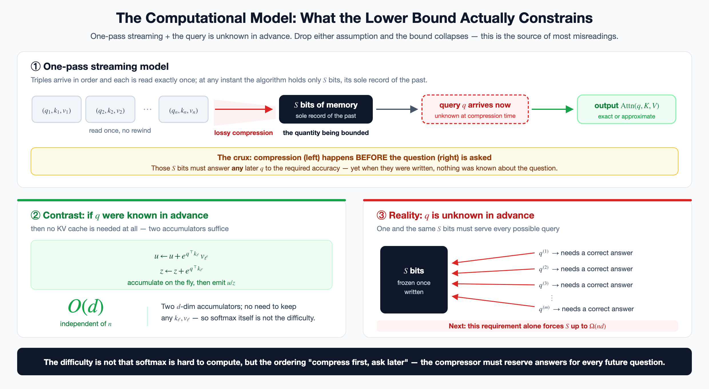
2.2 The ineliminable O(T)?
On this conjecture, I later searched the literature and found that the paper 《Compression Barriers in Autoregressive Transformers》[1] already treats it in detail. Specifically:
Some readers complain that too much math is “inhumane”, so here is the proof sketch in plain language: the problem is reduced to a communication index problem — that is, we view Attn itself as a memory-access problem.
- Alice holds a bit string ;
- Bob holds an index , and Alice does not know ;
- Alice may send Bob a single message (one-way communication, no interaction);
- Bob must, with probability at least , output .
The one-way randomized communication complexity of this problem is.
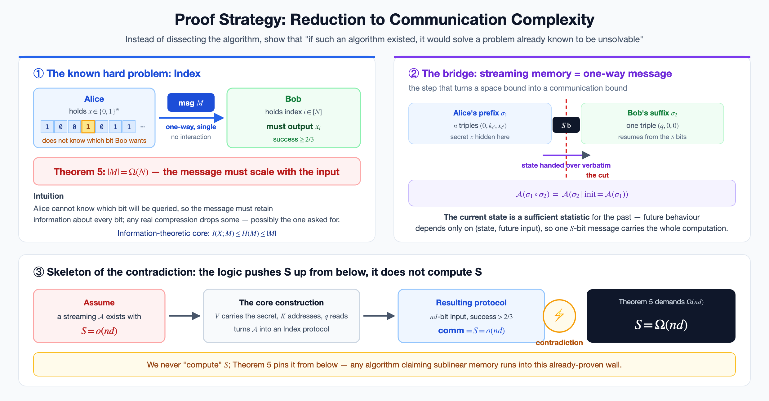
By analogy with Attn: Alice's input here is a 0/1 matrix , totaling bits; Bob needs to query its -th bit. Here is the token sequence length and is the hidden-dim. Attention is then used as an address-based read operation. We focus on Alice's KV encoding:
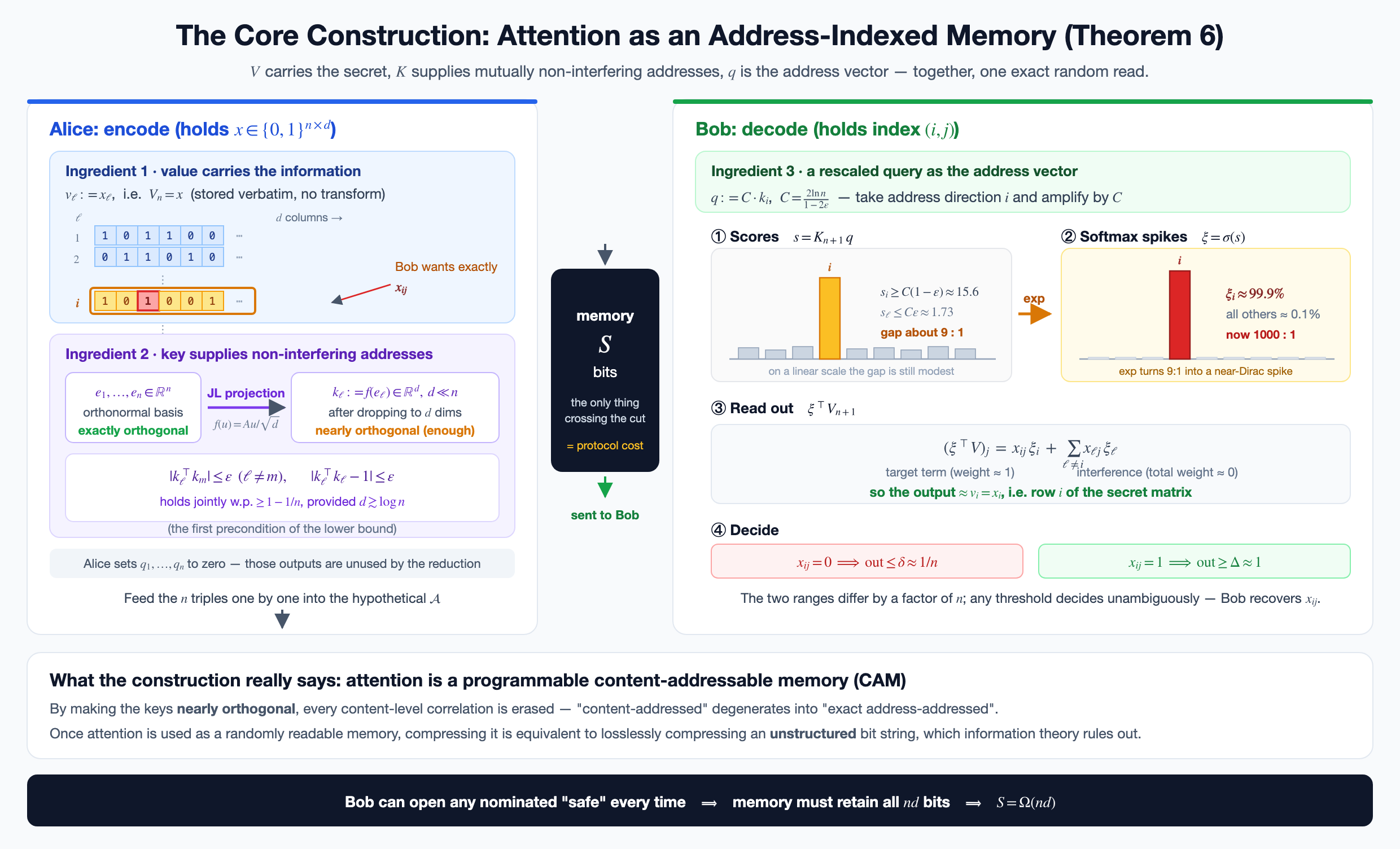
1. Values carry the information to be encoded: the most direct step — take 's -th row as the -th value vector:
2. Keys serve as mutually independent addresses: we need mutually non-interfering address vectors. In this is trivial: the standard orthonormal basis has pairwise inner products . But we want to compress the key space, e.g. keys live in a -dim space with , which cannot hold strictly orthogonal vectors.
This is where the Johnson–Lindenstrauss (JL) random projection comes in; it answers a beautiful question:Can we compress many high-dimensional vectors into low dimensions while approximately preserving all pairwise Euclidean distances? The answer is yes.
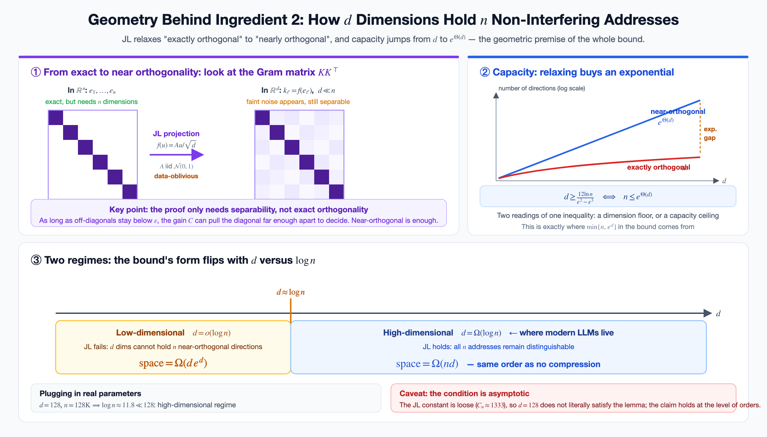
After Alice has fed in triples, she sends the -bit memory state to Bob. Bob then only needs to feed the algorithm one more triple , where
— i.e. take the direction of the -th address vector, scaled by a factor (this scaling trick is from Keles et al., 2022). The score vector then satisfies
This is exactly what the paper calls softmax's malleability: increasing makes and the remaining arbitrarily far apart, and the exponential amplifies the gap further, degenerating softmax from a smooth weighted average into an approximate argmax — a Dirac-like spike on the discrete support.
Let be the softmax weights. The -th component of the output vector is
(The row Bob fed in satisfies and contributes nothing to the numerator; only adds one term to the denominator, without changing its magnitude.)
Two cases follow. Denote the main term and the upper bound on the sum of interference terms :
Case 1: . the numerator keeps only interference terms, each , so
Case 2: . the numerator contains at least the main term itself, so
For the protocol to work, Bob must be able to distinguish these two intervals, i.e. . And
Any works. The paper takes , , which gives
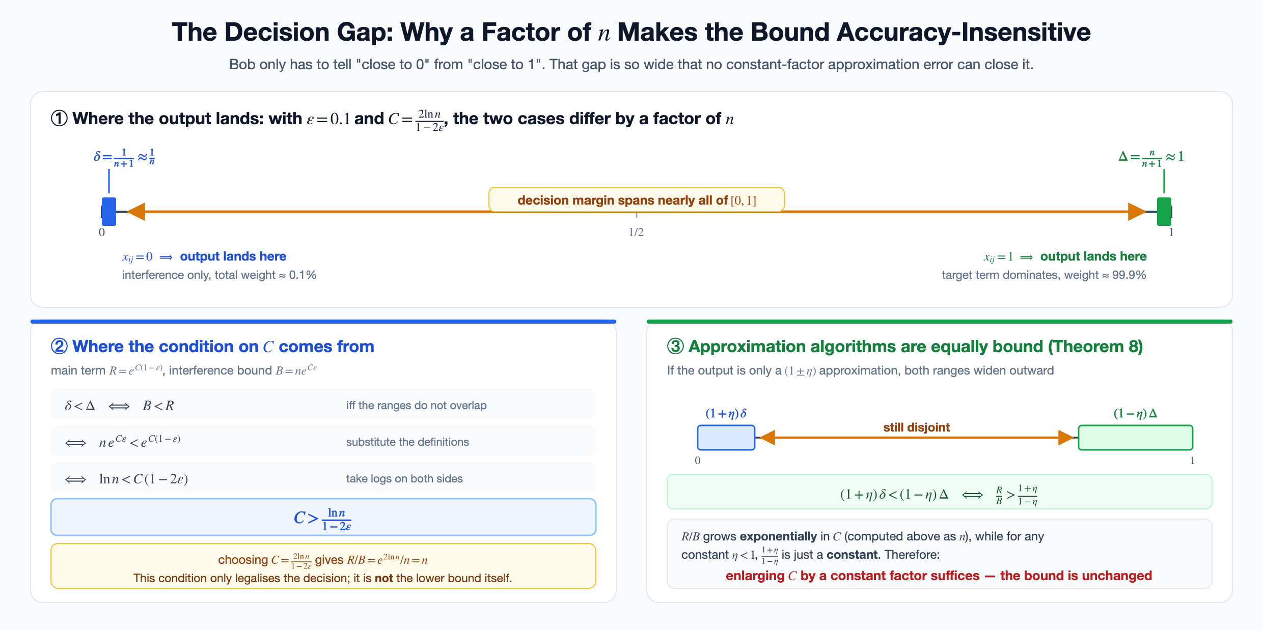
That is, the outputs in the two cases differ by a factor of . At this point the construction is complete, and the range of is fixed. But only guarantees that Bob can answer correctly; between that and “ must be large” there is still the entire finishing stretch of the reduction. The crux is that the protocol's success rate meets the requirement; there are two failure sources: the JL projection failing the inner-product condition (probability ), and the algorithm itself erring (probability ). Taking a union bound, Bob's success probability is at least
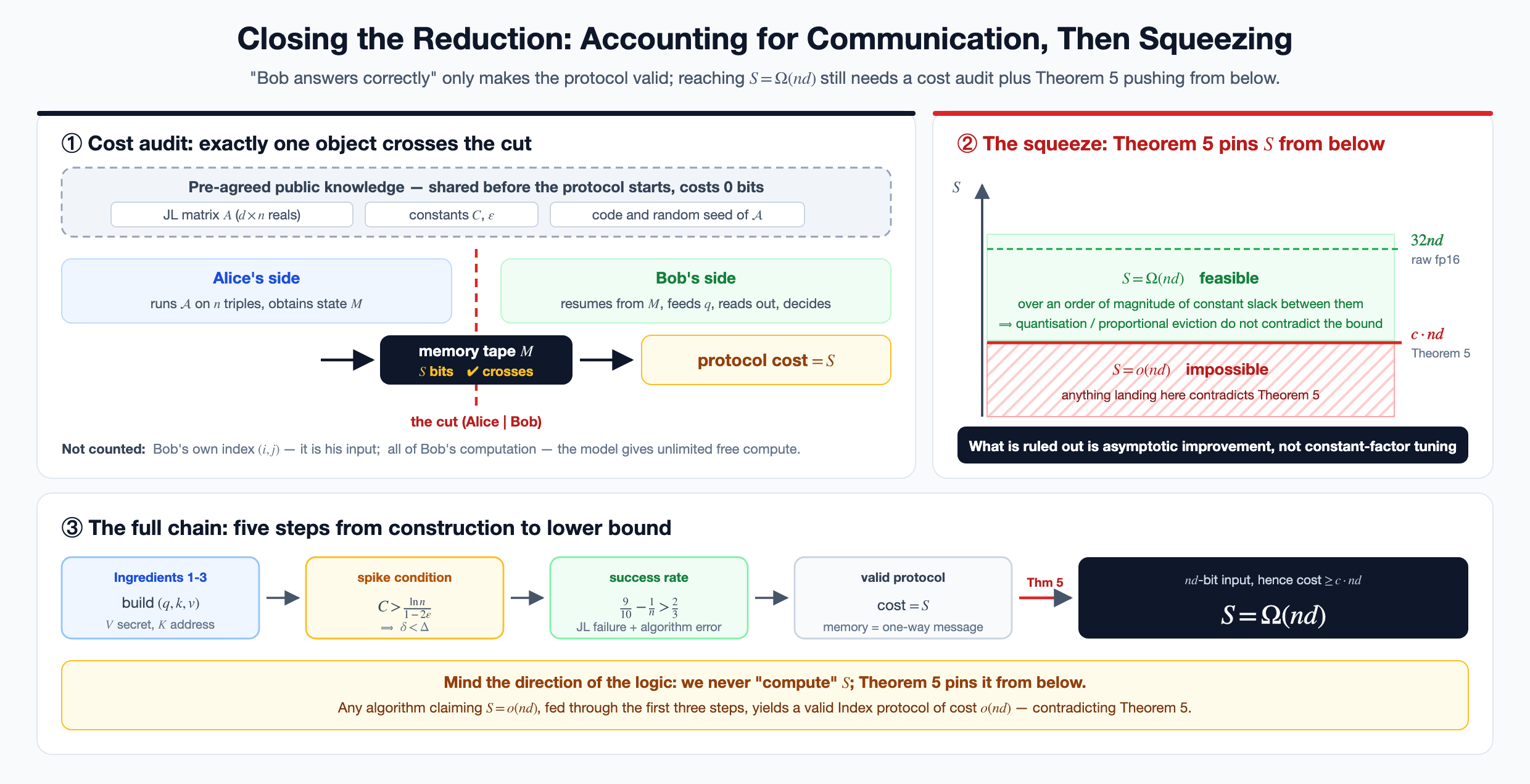
which meets the success-rate requirement of the index problem. At this point we hold a complete, valid protocol for the index problem:
- Input size: , i.e. bits;
- One-way, randomized, success rate ;
- Communication: .
The JL theorem asserts: any protocol satisfying the above conditions has communication . We can thus sandwich out the lower bound
The paper also discusses the following:
- The boundary in low dimensions: When the embedding dimension is small (), the paper proves a space-complexity lower bound of , and points out that the SubGen algorithm proposed by Zandieh et al. achieves this theoretical lower bound in this specific scenario. But typical LLMs today
- The role of structural assumptions: The paper explicitly states that unstructured sparsity alone is not enough to break the linear space barrier. In other words, merely knowing that the attention matrix is sparse, without knowing where the sparsity lies, still cannot achieve sublinear space. This provides a theoretical basis for many practical algorithms that rely on specific sparse patterns (e.g. sliding windows).
- Extension to sliding-window attention: The paper analyzes a more general sliding-window attention mechanism in which Value vectors outside the window are not completely ignored. For this scenario, the authors propose a novel sublinear-space algorithm based on reservoir sampling, and prove its space complexity is nearly optimal.
- Time-complexity lower bound: The paper also studies the time complexity of token generation, proving that any non-adaptive streaming algorithm (i.e. one with the data-access pattern fixed in advance) requires, in the worst case, at least .
2.3 The Linear vs Sparse debate revisited
In fact, a common rebuttal immediately arises here:
- Linear attention's state is fixed at , independent of , so it necessarily loses information and cannot reproduce the output of softmax attention;
- so it is a lossy approximation without any guarantees;
- so it is pointless — since cannot be dodged anyway, better to honestly store the full KV and then compress the KV dimension via the JL lemma — like MLA/DSA/CSA?
A fixed state is Linear Attn's biggest weakness: linear attention's state is times smaller than (taking , , about 2000x), so it sits completely outside the lower bound — supporters of Linear Attn have nothing to deny here; the first article already discussed the 9 defects of pure Linear Attn...
Of course such a conclusion is somewhat one-sided, because the Linear Attention path has already evolved into Hybrid Attention — e.g. should Kimi K3's block of 3 KDA layers + 1 Gated MLA layer be viewed as a whole?
For example, the hard problem used in the reduction is an index communication problem: Alice hides a bit and Bob later specifies a position to retrieve. This is essentially needle-in-a-haystack: exact retrieval of a single point from unstructured long context. So the theorem does not just say “sublinear must be lossy” — it pinpoints on which tasks the loss occurs. And this matches empirical observations: Kimi K3 may drop points on long-context exact-recall tasks, while losing very little on highly redundant tasks like language modeling, summarization, and commonsense reasoning. So is the whole K3 block (3x KDA + 1x MLA) itself a decent Attention structure? Hence a head-on opposing view: “My favorite kind of approximation is allowed to be lossy, yours is not” — and I don't need “guaranteed losslessness” either; being a bit blurry and appending a Full Attn afterwards is perfectly fine?
On the other hand, the paper also shows that without data-awareness, merely knowing the attention matrix is sparse — without knowing where — still cannot achieve sublinear space, which seals off a family of Sparse Attn algorithms without an indexer. For Hybrid Attn, Linear Attn supporters might also argue: the state matrix is a data-driven compression, the interleaved MLA restores long-range memory, and it adds many layers of inductive-bias capability over Sparse Attn, which could improve generalization?
So the Linear Attn vs Sparse Attn debate has shifted to Hybrid Attn vs indexer-carrying Sparse Attn schemes like DSA/CSA.
2.4 The Linear Attn perspective
2.4.1 A history of patches
The previous article “Kimi K3's KDA (1): How KDA Works with Gated MLA and AttnRes” also discussed in detail: various issues of Linear Attention mean must be repaired with a conv; then got added, had to be added too, and after that a nonlinear SiLU — the exponential computation one hoped to save crept back in; even so, the state still accumulates and collides.
Then Linear Attention could only keep writing into the state matrix with no way to forget. So Mamba-2 introduced — an input-dependent memory lifetime — but the forgetting was too coarse-grained and writing was still additive. Then came DeltaNet, i.e. , which can directionally rewrite along the current key, but lacks a mechanism to quickly clear stale global state. So Gated DeltaNet was built, i.e. , combining global forgetting with directional rewriting, but each head has only one decay. Then KDA appeared, , introducing an independent decay per key channel — but a fixed state still does not equal full token-addressable memory.
We then continue examining the transition . It has eigenvalues equal to , and the eigenvalue along the direction is Without constraining , even if , one can still get , causing that direction to be amplified or overshoot backward in the recursion. Then more patches: Q/K need L2Norm; the output gate also needs a full-rank projection, and MLA needs to be added as well — activated parameters grow by another 8B.
This is at the KDA operator level; further, from its algebraic structure, it is an affine contractive semigroup. The contractive property determines its limited ability to remember long-range retrieval, so Hybrid Attn must be used, with Full-Attn MLA as the supplement. This is how Linear Attn gradually evolved into KDA — a history of patches.
2.4.2 KDA's unavoidable walls
If we consider a future Linear Attn that can avoid full-Attention layers like MLA with O(T) KV and still gain sublinear benefits — equivalently, if we connect token-to-token attention into a topology, the question to answer is: can the “edge” between two tokens at distance survive in the KDA state until it is read out?, KDA's weights decay along time as , so the strength of this edge drops exponentially with distance. Set a “still alive” threshold (below 1% counts as dead), giving
The key is that making large has only one way: push toward 1. And triggers three bad things at once:
Wall 1: the requirement itself is extreme (the decay wall) : means grows 10x, must shrink 10x. can only support 458 tokens; to support 1M you need . , accurate to the 7th decimal place.This demands pinning a number at an extremely narrow spot in the neighborhood of 1.
Wall 2: the gradient at that spot is almost zero (the trainability wall): ; differentiating gives . To have you need — the far-left end of the sigmoid, approaches zero, a gradient four orders of magnitude smaller — effectively telling the optimizer “don't go this way”.
Wall 3: even if learned, it cannot be computed accurately (the numerical wall): §2.3.8 of the previous article also covered this — FP32 at has only 7 significant digits left, i.e. the long-range Attn topology loop at 1M distance is already unreliable in FP32.
The crux of the three walls is “mutually independent, tightening in the same direction”
All three are stuck on the same knob, and all worsen in the same direction; no setting of can satisfy all three at once. On the other hand:
- decay's lower bound is sealed (, cannot forget fully in one step) — this buys numerical safety, and the lost “fast forgetting” ability is compensated by the delta term;
- decay's upper bound is open (, long memory) — this buys expressivity, at the price of losing the uniform contraction gap.
But each delta step can only erase one direction (Rank=1). So: selectively clearing a -dim conceptual subspace needs at least steps. Decay can clear fast but has no within-channel selectivity. Forgetting that is “both fast and selective” is unreachable in a single layer at a single step — it can only be relayed over multiple tokens or layers.Does this also imply that several consecutive KDA layers must cooperate, and that the whole model needs a deeper network? In fact the depth axis's efficiency is also affected. This produces a dialectical contradiction:
- To preserve ultra-long dependencies, the model needs to push some channels toward .
- To keep learning the timescales of these channels, the decay gate must stay out of the saturation region.
- To preserve ultra-long dependencies, the model cannot use low precision to improve compute efficiency.
- To balance the decay contradiction, the model potentially needs more layers, which also hurts compute efficiency.
Next comes an efficiency question — or let me phrase it differently: why is FlashKDA's chunksize = 16? In the formula, the division by is the Achilles' heel of the chunkwise form: is the cumulative product of 's retention factors, and its reciprocal grows unboundedly with intra-chunk distance. Under negative-Softplus parameterization, 16 steps of accumulated decay can get arbitrarily close to , and overflow is inevitable at finite precision.
Kimi Linear's countermeasure is to subdivide the chunk into 16-token sub-tiles: off-diagonal tiles can use Tensor Cores after computing relative decay in log space, but diagonal tiles must still be computed explicitly position by position, becoming the main bottleneck of intra-chunk computation. Kimi K3's solution is to eliminate the numerical problem at the source: once is floored,
the reciprocal renormalization factor is representable throughout, diagonal and off-diagonal tiles unify into dense Tensor Core GEMMs, and the slow path is deleted entirely. This also explains the three reasons FlashKDA chose :
- Numerical range: lands exactly within bf16's dynamic range, needing no intra-chunk rescaling tricks;
- Cheap inversion: 's inverse expands directly with a Neumann series, no further factorization needed;
- Instruction mapping: all math maps cleanly onto SM80 MMA (
m16n8k16) instructions, keeping the kernel simple and portable.
A nice way to put it is that it happens to match the common GPGPU TensorCore 16x8x16 shape — but consider another question: for DSA-architecture accelerators like TPUs, whose systolic arrays are usually 128x128 / 256x256, what should we do? The rough problem is shown below:
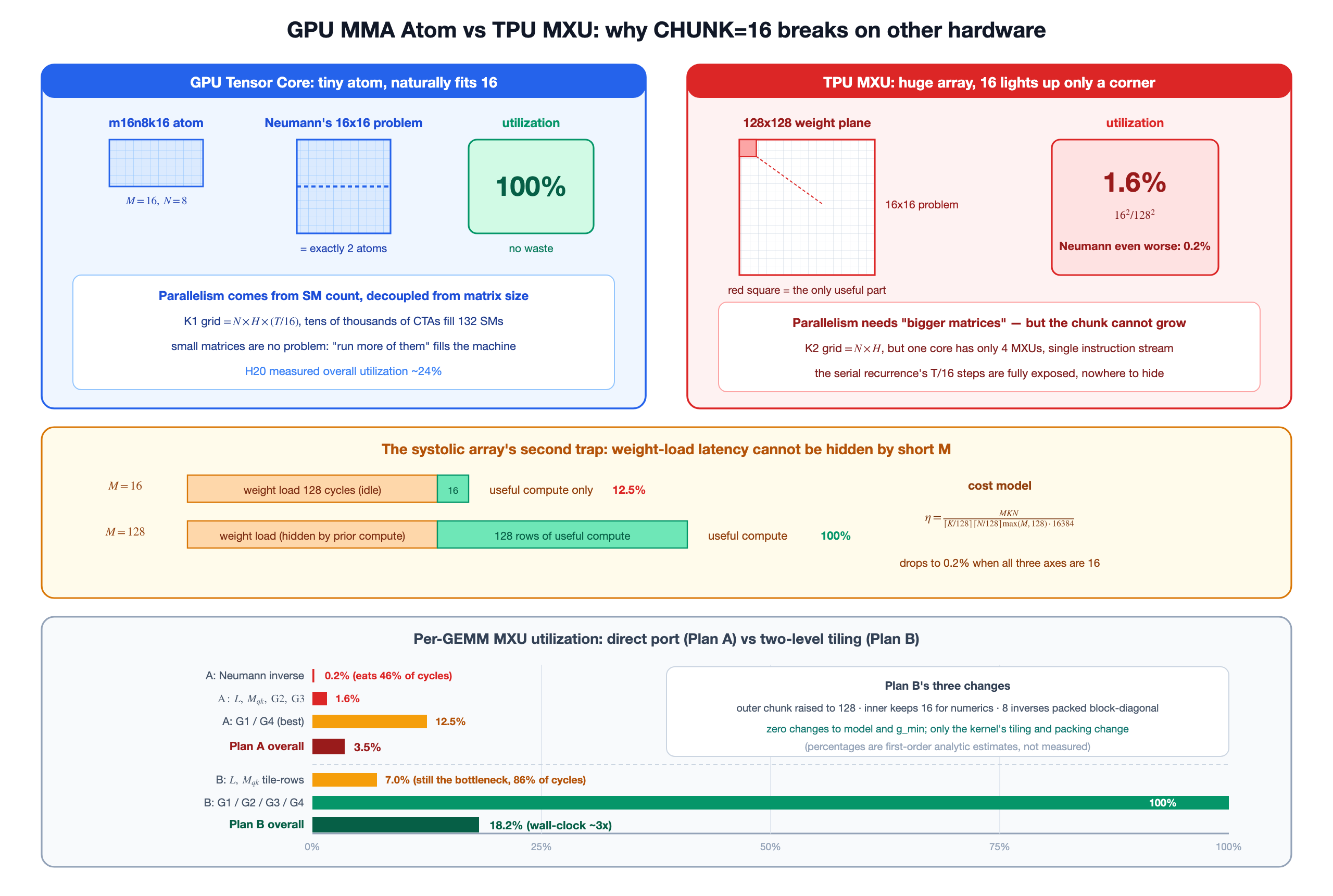
It looks like just changing CHUNK to 128 solves everything. But K3's numerical constraints bite back: single-level renormalization requires (both bf16 and fp32 have exponent ceiling ), so one cannot buy MXU-friendliness by raising — that changes the model, not the kernel. and CHUNK = 16 are a jointly calibrated pair.
The deeper obstacle lies in channel-wise decay: the dangerous factor appears inside the inner product
is a per-channel vector that cannot be pulled out of the dot product. With scalar decay like GDN / Mamba-2, is a pure scalar, free to re-anchor by block in log space, so enlarging the chunk is almost painless. KDA chose channel-wise for expressivity; the price is that the re-anchoring window is pinned by the numerical range to 16 token.
Of course we could also consider a 2-level loop tiling strategy: the outer CHUNK = 128 computes the GEMMs unaffected by at 128x128, and the inner uses concatenated matrices to improve TensorCore utilization. But overall the MFU would not be great either.
2.5 The Sparse Attn perspective
The Sparse Attn perspective is actually very straightforward: first, from the EOT viewpoint SDPA is the optimal solution, so softmax is worth keeping however slow. The remaining items: from the channel axis standpoint: acknowledge the sparsity of KV and compress the hidden-dim via the JL lemma — that is what MLA does. From the the token-sequence axis dimension: perceive the content to a certain degree and select through a lower-dimensional, lower-precision (FP4) evaluator (the indexer) — that is DSA. Another issue is that softmax peaks flatten as sequences grow: on one hand, attn-sink handling can be introduced; on the other, top-k selection also increases long-context kurtosis.
Then further blocking constructs the compression; and for the block-boundary jumping problem that top-k may have, overlap on the KV handles it — that is CSA. You can see DeepSeek's whole evolution here.
Of course, Sparse directly taking a constant topK may have problems: how to ensure that the blocks selected by this hard truncation can approximate Full Attn? A quick derivation:
For keys, sorted scores , softmax probabilities , where . Top-k truncation keeps the top and renormalizes: (), . Denote the tail mass .
: each head term gains (the denominator shrank); each tail term loses . The total “extra” of the head is , and the total “lost” of the tail is also . Hence
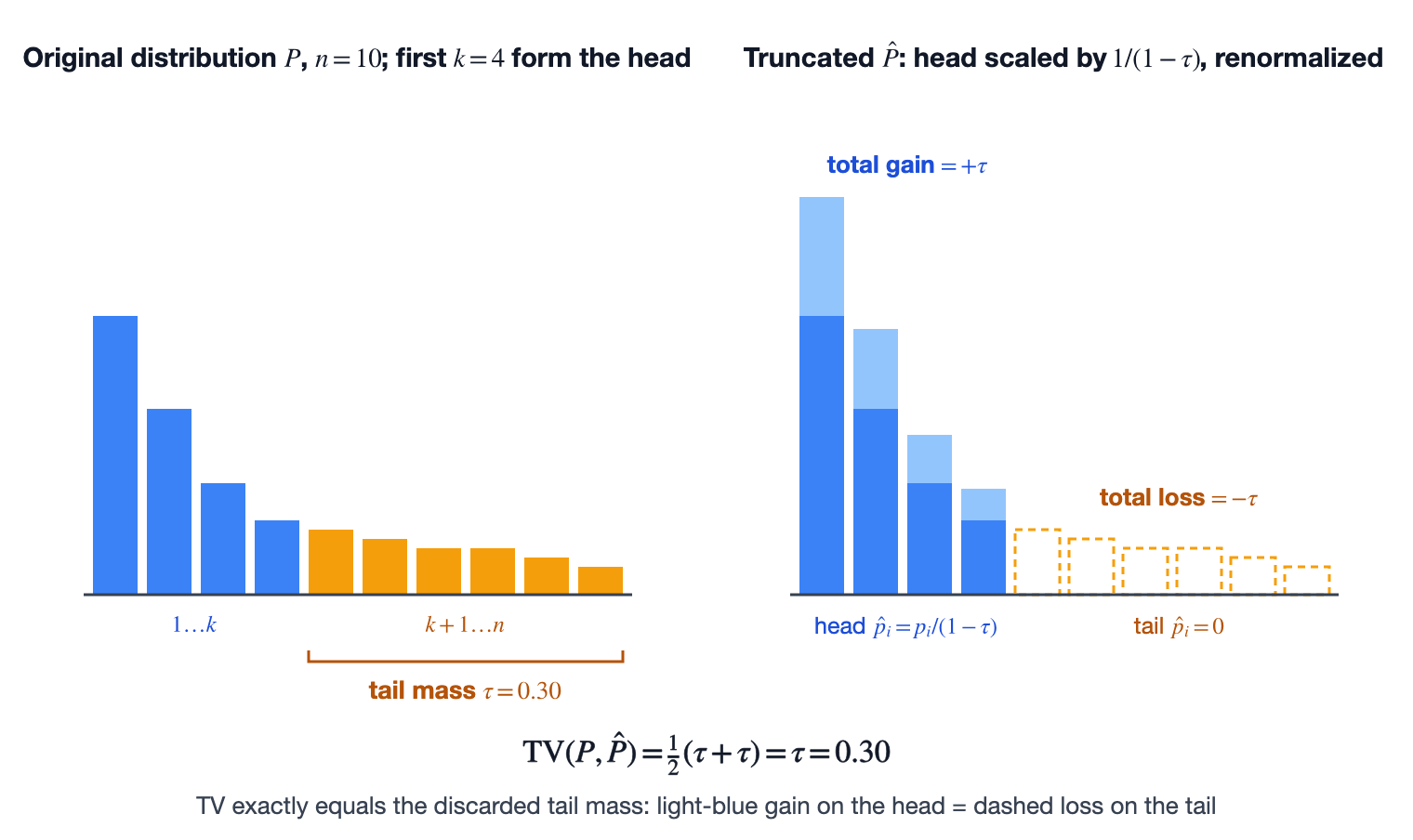
For , the likelihood ratio is a constant independent of . The expectation of a constant's logarithm is itself:
is a structure unique to Top-k renormalization. Now analyze the score distribution: each head term has , totaling terms; each tail term has , totaling terms. Substituting into :
that is, grows by 1, the error bound shrinks by about x. For example, at , , , which guarantees . This bound needs only two numbers.
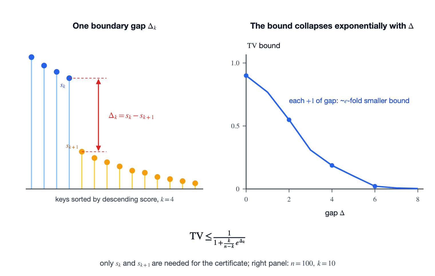
So to guarantee , from we directly get the single requirement:
Hence a simple bucketing algorithm:
- Bucket: while computing the score , also compute the bucket index , and increment the integer counter . Each key costs one subtraction, one rounding, and one increment.
- Table lookup: the keys in bucket are worth at most ; this table is data-independent and can be computed at compile time. “How many are in the bucket” times “how much each is worth at most” gives the bucket's mass upper bound.
- Accumulate: accumulate right-to-left starting from the rightmost (lowest-score) bucket, stopping as soon as the budget is exceeded. Whichever bucket it stops at, its boundary is the threshold ; keep keys.
There is another potential issue related to the HCA implementation: no matter how Sparse picks topK, how to further raise the compression ratio of a single block is also worth considering. HCA's pooling map is
Let us construct a minimal model: the gates are approximately uniform, i.e. ; within the window exactly one token carries the signal the query needs, , with scale ; the remaining tokens are mutually independent, zero-mean, same scale. The pooled slot is
The signal amplitude is , and the interference amplitude, by independent superposition, is . The of the two cancel, so the SNR takes an extremely simple form:
| Mechanism | signal | same-window interference | SNR | dB | |
|---|---|---|---|---|---|
| MLA | 1 | 0 | -- | ||
| CSA | 4 | 0.577 | dB | ||
| HCA | 128 | 0.089 | dB |
On the other hand, decompose the loss of the attention distribution via KL:
HCA's support set is all compressed slots, so the first term is identically zero for it: its read side is lossless, and all loss concentrates in the pooling step. This is actually the source of the defect: because the loss is entirely on the write side, and write-side decisions are query-independent, switching to another query buys nothing back.
3. Compression as Intelligence
As mentioned earlier, sublinear compression may have to be data-aware and data-driven. The KDA discussion at the beginning of this article is a great example: affine contractive semigroup — six words summarizing many of KDA's properties, yet current models do not seem intelligent enough for that... So for us, which compression directions should we consider at this stage?
First, I think we must admit the defects brought by overly pursuing Linear Attn, accept the current reality of , and then think about the following directions:
- the token-sequence axis: what is compressed is “how many tokens are kept”. Do multiple tokens need to form a block for block-based compression, or topK Sparse selection, or Linear Attn extensions, etc.
- hidden-dim channel axis: what is compressed is “how wide each token is stored”. Something like MLA, or potentially mapping different context segments into subspaces, e.g. Grassmann Manifold approaches.
- the model-depth axis: this is an axis that needs balancing, and the most easily overlooked one in comparisons. The query-awareness that Linear Attn loses in a single layer often has to be bought back with more layers, so the saved KV Cache is paid back as parameters, serial depth, and TPOT. So the real question on this axis is not “how deep can we stack”, but parameter efficiency per layer: can the same capability be obtained with fewer layers and fewer parameters?
- Chip-efficiency axis (an engineering axis orthogonal to the three above): can we compute at lower numerical precision? Dropping one precision level directly halves the constant term of while nearly doubling compute; another aspect is parallelization strategy — avoiding serial computation where possible, plus better data locality and kernel fusion.
- time axis This part involves Harness engineering: e.g. long-range context is easily lost, so is inducing the model to restate nearby content a balance point? Input tokens are relatively cheap, and parallelism on the Prefill side is easier for Linear Attn — but total inference time grows, trajectories get longer, and that is another trade-off to balance. On the other hand, data-aware anchors can be made during compaction to strengthen the selection of some blocks.
In essence, everything is about the memory-access optimization of the following formula
3.1 A Linear Attn that supports O(T)?
The conclusion of Section 2.2 is: if universal correctness for arbitrary future queries is required, the worst-case lower bound of fixed-precision storage is still bits. Traditional Linear Attention compresses the whole history into a single state, so all tokens compete in the same fixed-capacity matrix; Sparse Attention keeps addressable entries. Between the two there is another point worth studying: CSA/HCA sit in between at . However, HCA-style compression with 128-token blocks does not seem to be a very good scheme.
A natural idea: can we reuse Linear Attn's state-update method? Its expressiveness and order-dependence are stronger than simple pooling. So can we construct a new Block KDA algorithm that caches not every token, but solidifies one recurrent state every tokens, so that long-term memory grows from one global state into selectable states. — in short, Blockwise KDA splits one global irreversible bet into mutually isolated local bets.
There is another form, e.g. 《Log-Linear Attention》[2] adopts a Fenwick-tree hierarchy that grows logarithmically with sequence length to replace the single fixed-size state, keeping recent information at fine resolution and distant history as coarse summaries. There is also 《 Hybrid Associative Memories》[3], which builds hybrid memory and introduces a new HAM layer: tokens that are surprising for the RNN are stored as per-token KV, combining RNN and attention in a complementary way.
3.1.1 Constraints on block size
But numerical precision and the memory overhead of multiple heads and state matrices must also be considered. Let be the number of layers that actually enable blockwise KDA, be the bytes per element of the frozen state; each block additionally stores -dim routing anchors of bytes per element; for now assume different cache layers share this set of anchors. Without overlap, the cache is approximately
is the capacity-planning upper bound, including sealed archives and at most one hot-state allocation; online routing only scans the sealed blocks. So given a state-cache budget , ignoring rounding and tiny descriptor terms, the block size must at least satisfy
K3's 69 KDA state matrices stored in FP32 total 414 MiB; counting ShortConv and other activations as one full checkpoint, the upper bound is about 428.55 MiB. For a single sequence of , excluding descriptors and allocator metadata, the capacities for different are as follows:
| block count | 69-layer FP32 state | |
|---|---|---|
| 4,096 | 256 | 103.50 GiB |
| 8,192 | 128 | 51.75 GiB |
| 16,384 | 64 | 25.88 GiB |
| 32,768 | 32 | 12.94 GiB |
| 65,536 | 16 | 6.47 GiB |
| 131,072 | 8 | 3.23 GiB |
Another angle: based on the article's structure and common tokenizer estimates, we can use the following token-capacity tiers.
| Content unit | Common range | Recommended median | Typical composition |
|---|---|---|---|
| A paragraph | Token | Token | sentences |
| A section | Token | Token | paragraphs |
| A chapter | Token | Token | sections |
| A typical book | Token | Token | chapters |
Different types vary considerably:
- Fiction chapters are usually about Token.
- Typical non-fiction chapters are about Token.
- Technical-book chapters are about Token.
- Chapters with many formulas, code, tables, and references can reach Token.
So a reasonable block size is probably around 32K~64K.
3.1.2 Snapshots from Prefix Cache
There is actually a handy trick: KDA-style Linear Attention usually builds the Prefix Cache at the end of a request — see “When Prefix Cache Meets KDA: How Mooncake Supported Kimi K3 on Day 0”[4] for details. So we do have snapshots of the recurrent state per request. Could we then build some lightweight indexer to help the model pick a snapshot, or weight the top-k snapshots by some similarity with the query? This may require constructing a routing descriptor much smaller than the state, for the indexer to compute or for some weighting against the query.
3.1.3 Block overlap and fast/slow state updates
Blocks need some overlap to avoid semantic hard truncation between blocks. For example, with blocksize = 64K we can overlap by 32K: at Seq = 33K, it actually needs to update the state of the previous 64K block as well as the next window . This effectively forms a short-window fast-updating state based on (currently only 1K tokens), and a long-window slow-updating state based on (currently 33K tokens accumulated) — equivalent to a multi-timescale state matrix, which effectively increases the number of heads. Could the head count then be reduced accordingly?
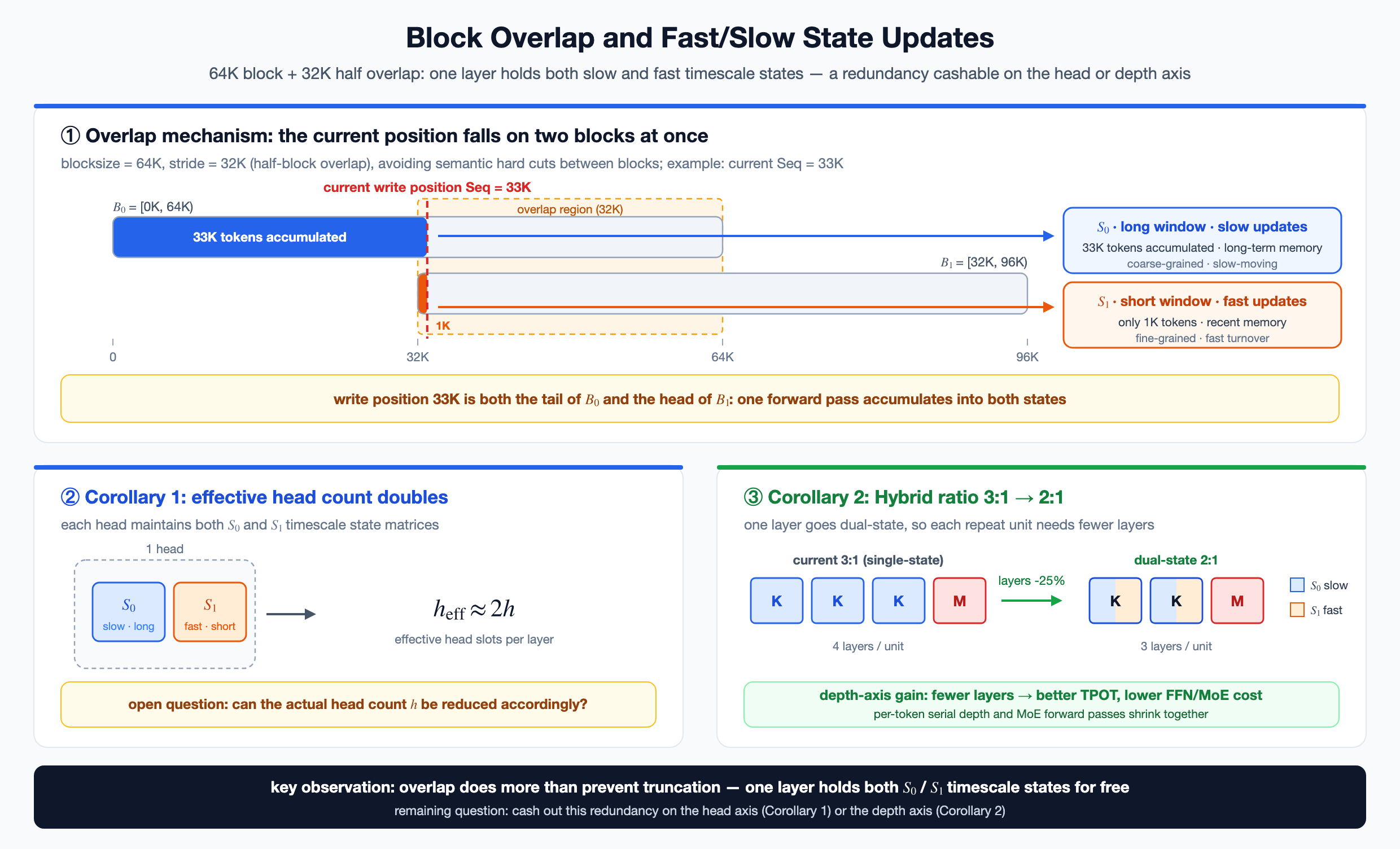
Or from another angle: since a single layer effectively has two different states being updated, can the Hybrid 3:1 ratio be further lowered to 2:1, buying back some TPOT on the model-depth axis and avoiding multiple FFN/MoE overheads?
As for compute cost, KDA is an affine monoid — which is exactly why the chunkwise parallel algorithm works — so the compute for overlapped states under the affine structure is not large.
3.1.4 Query-Aware block selection
At query time, given the blockwise state sequence , is there a TopK block-selection mechanism similar to Sparse Attention? E.g. use the query to compute block-relevance scores in a smaller-dim indexer, then take TopK? I searched and found that 《Memory Caching: RNNs with Growing Memory》[5] also discusses a similar problem.
A proper approach is to additionally store small anchors per block. To let multiple archive-enabled layers share one routing pass without creating inter-layer cyclic dependencies, let be the first layer that enables archive reads; before entering it, compute
and broadcast the same set of selected block IDs to the subsequent cache layers — or do block selection every few layers. From the chip's perspective, if later layers share the block IDs selected by an earlier layer, they also get better KVCache prefetch ability from CPU DRAM or external storage. Under the shared TopK routing scheme:
where is the forcibly retained set of recent blocks. After block selection, the outputs of hot and archived states can be mixed in a query-dependent way. Each state is already per-layer per-head; by default the mixing gate keeps this granularity too, but shares the candidate set :
where can reuse the shared routing scores, plus a tiny per-layer/head calibration term.
3.2 Hidden-dim compression via the Grassmann Manifold?
The previous section considered the token-sequence axis: organize history into still-addressable blocks, and let the query choose which blocks to visit. Another direction that can be orthogonally stacked on top is compressing the hidden-dim channel axis without merging tokens. First let denote the number of tokens in a block; the problem in the earlier HCA analysis is precisely that
it mixes tokens into one slot before the query arrives. Once the target signal and the same-window noise pollute each other in pooling, the read side faces a single indivisible object. A natural question follows: can we keep the independent addresses of these tokens, and only narrow each token from dims to dims, while letting different semantic blocks use different low-dimensional spaces? This is exactly the part the Grassmann Manifold perspective handles well. I previously introduced “[Math in LLMs - 103] Attention Algorithms from the Grassmann Manifold Perspective”
3.2.1 From the JL lemma to the Grassmann Manifold
Channel-axis compression has a ready-made classical starting point. What attention really needs is only the inner product , and the Johnson-Lindenstrauss lemma says precisely that inner products can be preserved by a low-dimensional projection: for any points in , there exists a map (and a random Gaussian matrix is one with high probability) such that
Two things make this conclusion attractive: depends only on and the accuracy , not on the original dimension ; and is data-independent — it can be chosen without seeing the keys, so it treats all future queries equally.
But plug in attention's scales and this path fails here. Take a block of keys; even requiring only a coarse accuracy like , is already in the hundreds, while our is only 128 to begin with; strictly speaking, covering arbitrary future queries needs a union bound or net argument over the query set, which only pushes larger. The JL lemma is designed for extremely large, scenarios; with a head dimension of just over a hundred, the budget random projection wants is wider than the original dimension — the compression ratio drops below one.
The reason is not hard to see: JL's guarantee is a distribution-free worst-case guarantee — it must hold for any point set, so it can only spread its budget evenly over all directions. Keys from a piece of natural language are usually not worst-case; they tend to concentrate near a few directions. To get real compression, we must give up the “data-independent” advantage and switch to data-adaptivity: replace the random with the principal subspace of this segment's own keys . The error then changes from JL's relative form to the actual residual (this bound will be used later in this section): when the low-rank assumption holds it can be far below JL's bound; when it fails, it honestly grows. A side consequence: JL preserves inner products, while the Value side needs to preserve the reconstruction of weighted sums — the optimal subspaces for the two are not the same, which is why K and V each learn their own basis later.
Once the projection matrix is changed to “chosen by data, one per block”, the representation gains an extra layer of redundancy to deal with — and this is where the Grassmann Manifold enters. What actually determines logits and outputs is only the projection operator , i.e. the subspace spanned by ; the same subspace has infinitely many orthonormal bases, differing by an . Quotienting out this redundancy leaves the set of all -dim subspaces
, namely the Grassmann Manifold, where is the Stiefel manifold. It gives this route three concrete things:
- Discipline: only functions of are legitimate gauge invariants, safe to use as scoring signals or cache metadata;
- A ruler: the principal-angle distance between two block subspaces tells whether they can share one basis, or whether similar blocks can be clustered into one tier;
- The correct optimization geometry: when learning , gradients should live on the Grassmann tangent space, rather than hard-updating numbers as free parameters.
Looking back from this perspective, several channel-axis compression schemes are actually the same thing taken differently; the difference is only “who chose this -dim subspace, and how many copies are paid for”:
| Method | Subspace from | Copies of bases paid | Assumption relied upon |
|---|---|---|---|
| JL random projection | Random, data-independent | 1 copy, or not even stored | No assumption, but the budget is not worthwhile at |
| MLA-style global latent | Learned in training, globally shared | 1 copy, inside the weights | The whole data distribution is approximately low-rank |
| The Grassmann codec of this section | Chosen by each block's own data | copies, stored with the cache | Each semantic block is approximately low-rank — a weaker assumption |
All three rows pick a point on , just moving from “a random point” to “a learned point”, and then to “one point per segment”. The further down, the weaker the assumption and the more local structure can be exploited, at the price of storing extra bases and one extra construction. It should also be said upfront: Grassmann itself produces no compression; it only accounts for the degrees of freedom and invariants of “choosing a subspace”; whether materializes depends entirely on how well the block-local low-rank assumption holds on real contexts.
3.2.2 From global latents to block-local subspaces
Let me first distinguish two levels of blocks: the 32K~64K block in Section 3.1 is the coarse-grained state/routing block; in this section denotes the length of the smaller subspace blocks divided by paragraphs or sections. Also, in what follows denotes the K/V channel dimension of the single attention head being compressed, not the model-wide ; if compression happens before , the same derivation can act on the full hidden-dim.
Let the representation of the -th subspace block be , and choose for it a set of orthonormal bases
, storing each token's coordinates in this basis
What really matters here is not any particular basis , but the subspace it spans. For any orthogonal matrix , and represents the same subspace, so a block's compressed object should be written as
The difference from HCA is immediate: HCA compresses rows into 1 row; a Grassmann block still keeps rows, each just going from dims to dims. The Grassmann point is only a block-local dictionary; is what holds each token's content, so one cannot store only and claim the whole block has been represented.
It can also be viewed as a context-adaptive version of MLA. MLA lets all tokens use the same latent codec learned during training; here, novel paragraphs, code blocks, and formula paragraphs may each pick their own local coordinate system. What is earned no longer presumes “the whole data distribution shares one low-dimensional space”, but the weaker “each local semantic block is approximately low-rank”. Correspondingly, each block also pays an extra of storage and construction cost.
| Mechanism | A -token block after compression | Addressable token count | Main information lost |
|---|---|---|---|
| HCA | 1 -dim slot | 1 | Intra-block detail on the token axis |
| MLA-like global latent | -dim coordinates | Channel directions discarded by the global codec | |
| Grassmann block | 1 set of bases + -dim coordinates | Orthogonal residuals outside the current block's subspace |
3.2.3 Sparse Attention inside local coordinates
The Grassmann Manifold itself saves no FLOPs out of thin air; the real gain comes from not up-projecting each token back to dims, but doing the attention of selected blocks directly in local -dim coordinates. Let an attention head's Key and Value dimensions both be . A safer default is to learn two subspaces separately
and cache, for each solidified block,
Here the Key subspace preserves query-key logits and the Value subspace preserves weighted outputs — the two optimization objectives differ; so strictly speaking, each block corresponds to a pair of subspaces on ;
First, the query's projected energy onto the Key subspace can serve as a block-routing signal:
It has two lovely properties:
- Gauge-invariant: under a basis change , the projection matrix is unchanged, so the score does not depend on the choice of basis and is well-defined on the Grassmann point .
- Cheap to compute: computing it takes just one projection, without ever touching the coordinate matrix .
But cheapness has a reason: it reads no coordinates, so it cannot see the content. Decompose the true logit of some token in the block along the subspace (denote ):
): the projected energy only gives a permissive upper bound on the first term: by Cauchy-Schwarz, . Large energy only means the block's dictionary directions align with the query, permitting large logits; whether any token in the block actually put content on those directions is determined by the coordinates , and never reads them. A block on the same topic as the query may well have a well-aligned dictionary while all its tokens' coordinates fall on directions nearly orthogonal to : a high score, yet not a single relevant token. So it only answers “does the query align with this subspace”; using it alone to rank blocks would produce systematic false positives. Its proper place is as one feature of the scorer, trained together with coordinate statistics and content descriptors.
The reverse — exclusion — can be made rigorous, but both terms must be controlled. The decomposition above gives a per-block logit upper bound
Here the two query-side factors come free from ; the two key-side maxima are scalars computed while the block is being sealed: the former is the maximum coordinate norm, the latter the maximum norm of the discarded orthogonal residual, and both cost just one scalar of cache. When this upper bound falls below the logit threshold of the current candidate set, the whole block can be safely skipped. Note the residual term cannot be omitted: the information for which the low-rank assumption fails sits exactly in ; excluding with only the in-subspace term would prune the needle hiding in the residual along with the block.
This nails down 's position in the routing stack: combined with blockwise Sparse Attention, the token axis and the channel axis each handle half, with a clean interface:
- Which blocks to read is decided by the content-aware indexer's ranking; is just one cheap feature of it; the inequality above serves as a safety pruning independent of the learned score, deleting blocks whose upper bound cannot reach the threshold. The feature may enter the scorer, the pruning is guaranteed, but neither can replace content scoring itself;
- In what format to read is decided by the codec: selected low-residual blocks do attention in -dim local coordinates, high-residual blocks take the raw bypass, and read bandwidth is tiered by rank;
- Costs are booked separately: scoring all blocks, whether by indexer or by projection energy (the latter ), is a linear scan; what the codec saves is the reading and compute of selected blocks, not the scan itself. To make the selection phase sublinear as well, hierarchical indexing or approximate retrieval is needed — orthogonal to the codec.
Let the final routed set of blocks be , and compute for each selected block
Here the denominator keeps the original attention's , because the goal is to approximate ; directly replacing it with would additionally scale the logits by ; if calibration is really needed in training, a learnable temperature should be introduced explicitly. Then a joint Softmax is still done over the tokens of all selected blocks:
where . The last formula is key: each block first aggregates Values in its own -dim space, obtaining a -dim vector, and only then is each block up-projected once and summed, rather than restoring all Values to dims. For any , under the transformation , the local coordinates rotate accordingly, and both logits and final outputs are unchanged. So this computation depends on the equivalence class formed by the subspace together with local coordinates, not on any particular basis; the Grassmann point itself contains no token content.
The formula also spares a trouble by the way: each block is up-projected separately, and the -dim coordinates of different blocks are never added directly, so no parallel transport or connection needs to be defined between them. That would only be needed if one wanted to mash the -dim vectors of multiple blocks into the same coordinate system before a unified up-projection — and the error it introduces may not be worth the few projections saved.
If the K/V within a block has a significant non-zero mean, each can store one more center and only the centered residuals are compressed — i.e. replace the linear subspace with an affine one. The cost: logits need an extra term , block outputs need an extra term , and each block stores more elements.
3.2.4 How much can it actually save?
If Key and Value each use a basis, a block's raw KV storage and Grassmann-coordinate storage are respectively
So the whole cache of length goes from to
The compression ratio is
For example, with , counting only elements, a block drops from KV elements to , a theoretical compression ratio of about ; if K/V share one basis it is .
Let be the number of blocks actually read per query after top-k and safety pruning; the main cost of low-dimensional reading is
Compare with the of restoring the original KV. Only when and the kernel can consume local coordinates directly does this gain approach . Also, as noted earlier, scoring all blocks one by one is still an linear scan, which needs hierarchical indexing or approximate retrieval to push down; and note that Grassmann projection does not make the token axis sublinear.
3.2.5 Only let “compressible” blocks enter the low-dimensional space
The derivation above implicitly assumes something strong: a block's K/V is indeed close to some -dim subspace. This may hold for repetitive natural-language paragraphs, but not necessarily for blocks containing multiple topics, rare entities, formulas, or code. Denote
The joint projection residual can decide whether a block should be dimension-reduced:
where balances the residual scales of Key and Value.
In practice, one can offer just hardware-friendly compression tiers, plus a raw -dim bypass. Choose the smallest satisfying ; each compression tier corresponds to one ; blocks of the same rank are batched together, and the blocks picked by top-k in one decode step are naturally bucketed by tier — one batched gather and GEMM per bucket, avoiding fragmented mixed-rank kernels.
If even at the residual is still large, take the raw bypass directly, split the block, or additionally keep a few high-residual exception tokens; there is no need to store an extra Grassmann basis. Note the separation of duties between tiers and selection: the indexer's score decides whether a block will be read, the rank tier decides how much bandwidth reading it costs; the former varies per query, the latter is locked once when the block is sealed. After the orthogonal residual is discarded, even if a block is later frequently picked by top-k, it cannot be temporarily upgraded from to unless the cache kept nested residuals or another high-rank backing store in advance. This is what “let some blocks be processed in a lower-dimensional space” really means, rather than forcing all contexts to accept the same compression ratio.
Looking only at average reconstruction error is still not enough. The error of a single logit introduced by Key projection satisfies
This means a fact with low variance that will be precisely queried by a future query may well hide in the orthogonal residual; once the residual is discarded when the block is sealed, no later query can recover it.
In causal inference, the currently unfinished block keeps a full-dim hot cache and does not enter the top-k candidate pool: together with the most recent blocks it forms the forcibly retained local branch, unconditionally entering the attention support set — consistent with the Sparse route's convention of keeping a local window. The block enters the pool only when it is sealed: build the indexer scoring descriptor, pick the rank tier by residual and convert to low-dimensional coordinates (or mark raw bypass), and cache the two max scalars for exclusion. Training must also only let early queries use blocks sealed before them, otherwise constructing bases or scoring descriptors with future tokens of the whole block would cause covert causal leakage. A safer cache is therefore three-tiered:
- The recent window and the current block stay full-dim, unscored, always-on;
- Low-residual historical blocks store , read only when selected by top-k, consumed in local coordinates;
- High-residual blocks and exception tokens keep a full-dim escape path, also read only when selected, just in raw format.
The three tiers differ only in storage format and read conditions — they are not three separately normalized attentions. The candidate set of one decode step is “forcibly retained local branch + top-k-selected blocks”, and the scalar logits from raw tokens and from low-dimensional blocks must be concatenated into the same set for one Softmax, otherwise each branch renormalizing separately before summing would systematically change the probability mass of the original attention. If an exception token is kept in raw form, it must also be removed or masked from the corresponding block's low-dimensional coordinates, to avoid counting the same token twice.
There is another issue easily masked by positional encoding: estimating subspaces directly on RoPE'd Keys, the rotation of the same semantic direction at different positions can artificially inflate the block's effective rank; the same rotation also pollutes the indexer descriptor, making two blocks with the same content at different positions look different on the scoring side. So a more reasonable ablation is to compare “compressing content Keys while keeping the position branch separate”.
Stringing the whole pipeline together: the token axis selects, the channel axis compresses. When a block is sealed, the rank tier (or raw bypass) is decided once, and three pieces of metadata are built: the indexer's scoring descriptor, the subspace basis and local coordinates, and the two max scalars for exclusion. At read time the query scores all sealed blocks, and after safety pruning and top-k we get ; the support set is the forcibly retained local branch plus : low-residual blocks do token-level attention in local coordinates, high-residual blocks and exception tokens take the raw path, and all candidates are concatenated into the same Softmax.
3.3 Harness? Compression on the timeline?
The previous two sections focused on how to compress along the token axis and the hidden-dim channel axis within a single forward pass inside the model, but there is another dimension — the time axis. Especially in Agent runtime scenarios, user messages, Agent outputs, tool calls and results, checkpoints, etc. keep accumulating into an ultra-long context; which history should be fed back into the model in the next round?
The DeepSeek Harness paper 《A Programming Paradigm for Spatiotemporal Composability》[6] is about Agent Harness, but I believe the Memory in the model's own inference process likewise needs some local temporal/spatial composability structures.
The paper promotes effect and coeffect to runtime mechanisms:
- Reversible effect Each context transformation carries an explicit inverse tracked by the runtime, and both tracking and restoration preserve composition, so the context is restored when the component is removed. This establishes local temporal composability.
- Responsive coeffect A component declares the coeffects it needs as a specification, and every change of the context notifies the component against that specification. This establishes local spatial composability. Then the effect context and the coeffect context are unified into a single context type, where observation on coeffects provides independence for effects, forming a programming paradigm of spatiotemporal composability.
This corresponds exactly to the two questions we ask on the time axis: can the compressed-away history be withdrawn, and who should be notified to recompute after compression .
3.3.1 The timeline is actually three clocks
Treating “the timeline” as one axis is the easiest mistake here. There are actually three clocks ticking independently:
- The token clock, usually determined by the position order within one forward pass, which this article analyzes separately as the token axis
- The session clock, usually driven by interaction rounds, compaction generations, and branches — the subject of this section
- The model clock, caused by dynamic changes of weights, tokenizer, engram, etc. — the most easily overlooked. Inference usually assumes frozen weights, but as we gradually evolve toward Test-Time Training (TTT), these changes must be considered simultaneously.
For example, a common TTT practice builds an “inner loop”: by optimizing a neural network (e.g. an MLP) on previously observed tokens, it dynamically builds a temporary KV mapping. Subsequent inference steps are viewed as querying this stored knowledge. E.g. Titans: Memory as context — we can build off-path parameters through which query vectors produce a new block appended to the KV context before entering the Attention block, with updates possible at the output and residual parts too.
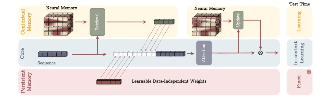
In essence, the macroscopic result TTT brings is the time-variance of the model's parameter weights. With the clock perspective, a direct corollary is that KV is materialized under a set of configurations:
where is the effective parameter of the TTT weights, is the storage and decoding convention. And from the paper 《Test-Time Training with KV Binding Is Secretly Linear Attention》[7] we can see that TTT-KVB is essentially a Linear Attn, so it can be discussed within a relatively unified yet opposing Sparse / Linear Attn framework.
3.3.2 Compaction! Compression of the timeline
For KV Cache handling, from a database engineering intuition, the tokens output by Decoding and the KV needed for speculative-decoding verification naturally suggest building something WAL-like token by token. And given the actual storage hierarchy, many Agent Harness frameworks use compaction for long contexts — is that also analogous to LSM?
From an engineering view, a storage system must satisfy two things at once: writes must be immediately persisted and must not corrupt, and reads must be able to locate a key quickly. These two are naturally opposed:
- For reads to be fast, data must be ordered and clustered. So every write has to be inserted at the right position, producing random I/O and in-place modification of a large structure.
- The most dangerous thing about in-place modification is not slowness, but data corruption under anomalies. If power is lost halfway through a page write, the structure is neither the old nor the new state, and afterwards one cannot tell whether to roll back or to finish forward.
WAL and LSM trees are the two halves of the answer to this conflict: WAL answers “this indeed happened”; LSM trees answer “how what happened should be arranged for reading”. Mapping it to an Agent's session history, we essentially need the Attention algorithm to support the following capabilities:
- Per interaction: the per-token WAL obviously exists for Sparse Attn, while Linear Attn needs State snapshots per interaction round.
- When building compaction, can it be built in an LSM-tree-like way? E.g. build a dedicated tombstone token — or call it an anchor token — for addressing, so the corresponding block can be indexed quickly. Per-token data is also compacted block by block.
- The whole context is composed on demand at block granularity (Composable ctx), i.e. different blocks can be swapped.
3.3.3 Algebraically, who is invertible and who commutes?
A common saying is that Full Attn / Sparse Attn is append-only on the time axis and therefore invertible and commutative, while Linear Attn pays these two properties for the ability to forget. The direction is right, but separating invertible, commutative and compressible or not — these three things — leads to much more interesting conclusions. The key is distinguishing the algebra of the write side from whether the read side has a length-independent exact summary:
| Mechanism | Write-side algebraic structure | Inverse exists | Commutative | Length-independent exact summary exists |
|---|---|---|---|---|
| Full / Sparse KV | Free commutative monoid (set union) | Yes — delete entries or roll back the watermark | Yes | No |
| Ungated linear attention | Abelian group (vector addition) | Yes — subtract the term | Yes | Yes, |
| KDA / GDN | affine contractive semigroup | No | No | Yes, but merging must preserve order |
The first and second rows happen to be complementary — a point worth noting:
- The write side of Softmax KV is a perfect WAL (append, commutative, deletable), but its read side has no query-independent exact summary whose dimension is independent of the block length — and this is the root of why lossy compaction is truly hard.
- Ungated linear attention's both associates and commutes — two blocks can be merged exactly, which is precisely the algebraic structure LSM-style compaction needs; the price is no forgetting, so it hits the walls of capacity and interference.
KDA is the only one that loses both: the inverse does not exist because contraction is non-surjective; it does not commute because multiplies the entire state. So handling KDA on the whole model's forward path in Agent scenarios is still somewhat complex — at least achieving equivalent reversibility between short rounds requires keeping some snapshots.
4. Summary
Prof. Tang's recent 《Memory for Large Language Models》[8] article classifies them from the perspectives of persistence and representability:
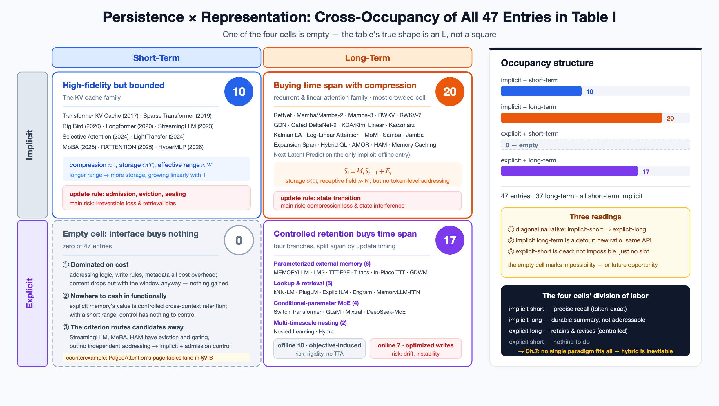
From the survey's literature statistics, the Linear-Attn-represented implicit + long-term route has developed rapidly in recent years:
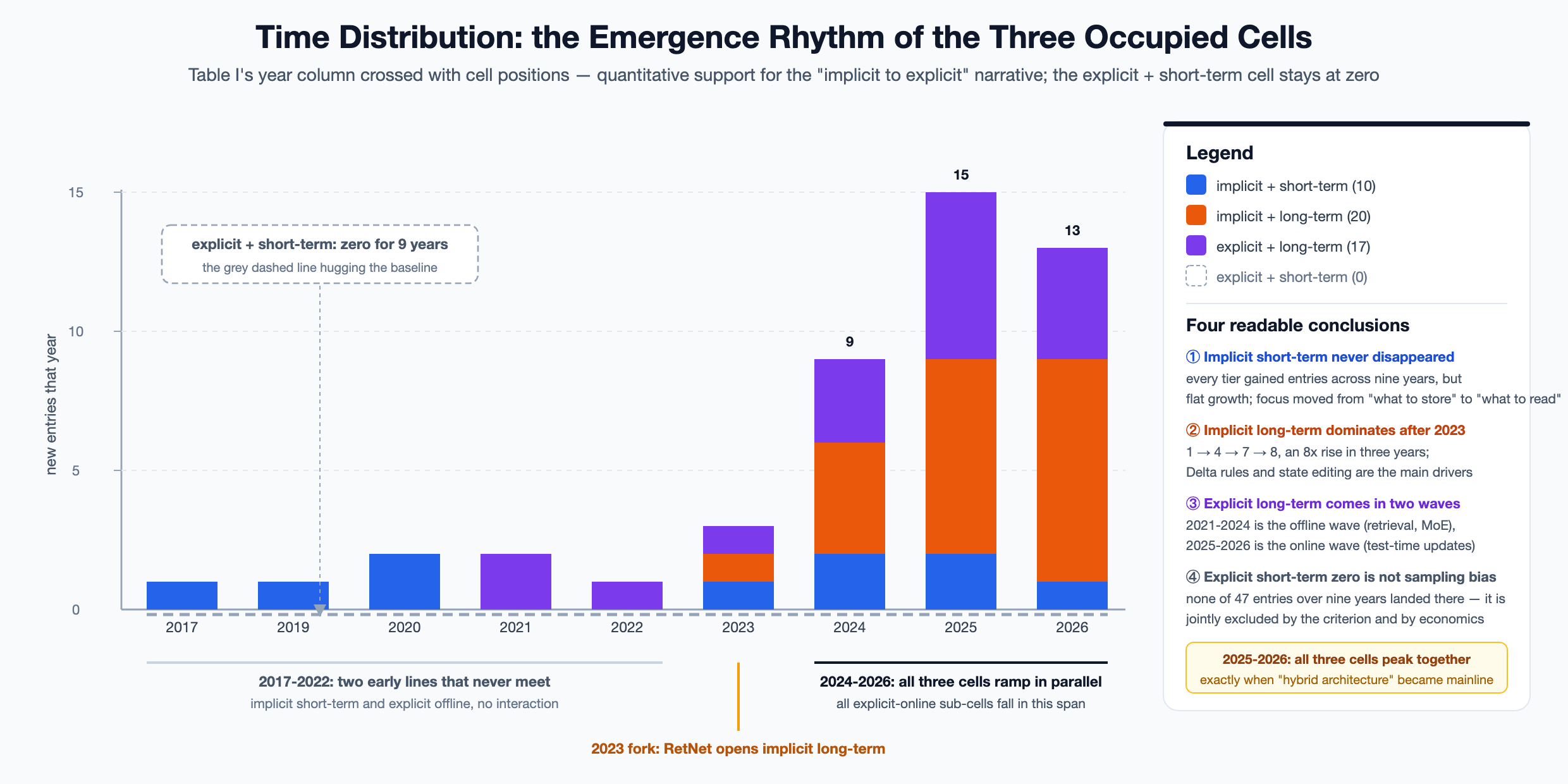
But note that it essentially compresses through the state matrix, buying better time-span representation — a natural state summary of sorts. The price is per-token addressability and commutativity/reversibility over the context. On the other hand, the explicit + long-term path is also developing rapidly; TTT in particular and future RSI-related developments deserve attention too.
So the questions explored in Chapter 3 have two sides: on one hand, migrating KDA-style Linear attn from implicit + long-term gradually toward explicit + long-term. On the other hand, how Sparse Attn can do more effective session / ctx compaction.
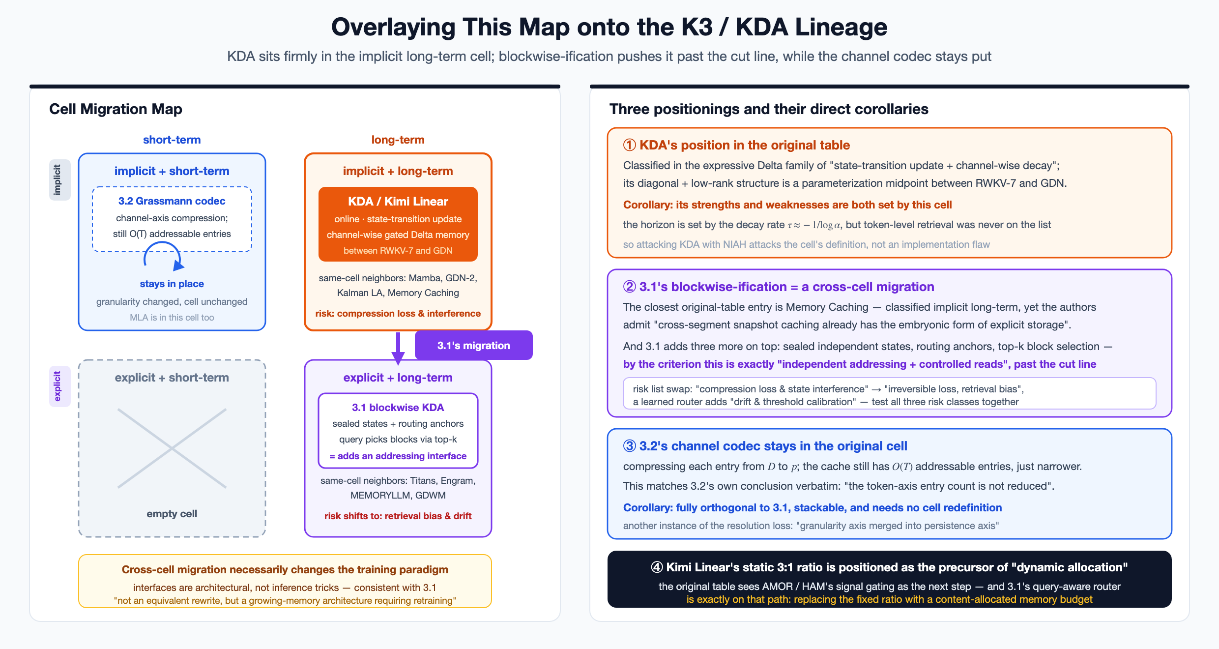
A more detailed architecture-perspective expansion may come later — e.g. treating Linear Attn State as a kind of Register File, Sparse Attn's KV as a kind of Dcache, and Attention itself as a kind of Control Unit, with MoE / Engram as a kind of addressable external storage.
This article is long enough; more details later when there is time...